matplotlib via L3

1 Get some data

The following scripts and data will produce several files in the current directory, so creating a new one for this demo is a good idea:

   mkdir l3demo
   cd l3demo

Start the gui via

   l3gui

and look for section 1.B, "Short Examples", on the left side. Left-click on "1. collect finance data", center-click on the right drawing canvas to paste the outline, and left-click the arrow twice to expand the script.

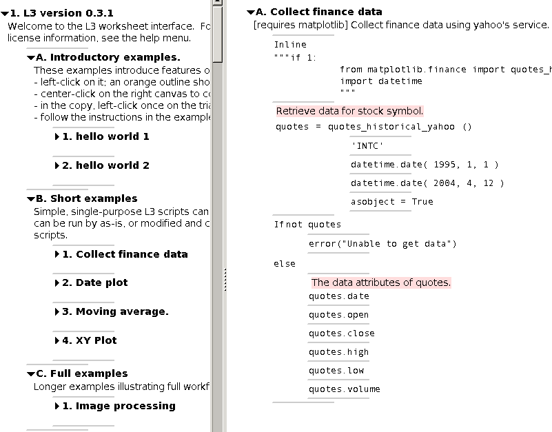
In the script the most relevant parameters are accompanied by highlighted comments, allowing us to focus on them and ignore the rest of the script for now. Looking at the first set of parameters, the stock symbol INTC (Intel Corp.) can be found at, e.g., yahoo finance. The start and end date range are fine as-is, and the asobject parameter can be ignored.

Run the script to get the data: right-click on the header ("A. Collect finance data") and select run code. If everything worked, the console displays some output we can ignore, and the last expression (quotes.volume) is highlighted in the gui.

2 Select data of interest

We want to see something, namely opening price for a given date, or a graph of quotes.date vs. quotes.open. To copy quotes.date, left-click the . (period) to get an orange outline around both parts of the name, and center-click on the canvas to copy quotes.date. Do the same for quotes.open, and your canvas should look like the following image.

3 Display the data

The chosen data (quotes.date and quotes.open) is next given to a plotting routine for display.

First, reduce clutter. Collapse the finished Collect finance data block via another click on its triangle.

Next, copy the Date plot script from the left library pane (section 1.B.2), via left click on it followed by a center click on the right canvas. Expand Date plot via two left-clicks on the triangle.

Again we see highlighted commentary. Your display should look similar to this one.

The plot details can be ignored for now, so we can hide them. Right-click on Inline (below Plot details) and select hide from the menu.

Our plot data needs to replace the defaults. Using the left button, click and drag the List of dates over to the right (out of the plot_date call), then drag the List of values the same way. Then insert quotes.date by selecting it (left-click on the period) and center-clicking the grey separator bar below the File name (the grey separator magnifies when the mouse pointer is above it). Insert quotes.open below quotes.date in the same way. After swapping the data, the canvas should look like this.

Clean up the List of dates and List of values via right-click and selecting delete.

To form the plot, right-click on Date plot and select run code. After this finishes, quotes.open will be outlined and the plot file name will show on the console, e.g.

   ('_plot-33081.png', 57)

To view the plot, right-click filename and select .png -> insert (file path, image) list to get something like the following.

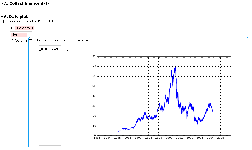
View the plot and when done right-click on File path list for `filename` and select delete.

This explicit sequence of

1. assembling a plot script
2. running it
3. viewing the graph

is more tedious than simply selecting the data and clicking a "Plot this" button, but it is also far more flexible. This flexibility is used next.

4 Save and load session

To safeguard the work, or to simply continue later, use the menu File > save session to, and choose, e.g., st.1 as file name.

To restart where we left off, start a new gui using the saved session via

   l3gui -s st.1 

in the console.

5 Filter the data and display

The data shown is really just

    plot(quotes.date, quotes.open)

but it is very jumpy, so next we want to view a smoothed version

    plot(quotes.date, smooth(quotes.open))

For this example, a simple running average is used.

First, collapse the Date Plot outline (click on the triangle).

Then make a copy of Moving average from the left canvas (entry A.2.C), insert it below Date plot, and expand it.

Below this Moving average, put a COPY of the previous Date Plot and expand it. For both, first select via left-click, and paste copy via center-click.

To adjust the Moving average data, again follow the highlighted outline, replace the Data with a copy of quotes.open and change the averaging interval to 30. To make this change, double-left-click the number 2, and in the edit expression window, type 30 and click Ok.

To adjust the new Date plot data, replace quotes.open with a copy of mov_avg. After these changes, and before cleaning up the garbage, the canvas should look like the following.

Now, compute the moving average via right-click on Moving average followed by run code, and run the new Date plot similarly. Then, delete unused expressions (numpy.array and quotes.open), collapse the finished Moving average script, and expand the first Date plot script.

With both plot scripts exposed, we can now view both plots (via right-click filename and select .png -> insert (file path, image) list) to get the following.

6 Organize scripts and save session

There are now four scripts on the canvas that can be moved independently, and some data that can be redisplayed any time.

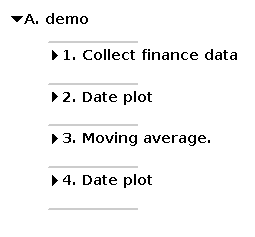
This can get tedious, so first delete the data. Then, copy an outline template from the left canvas (entry A.4.B), expand it fully (two left-clicks on the triangle) and insert the scripts into it (select each script via left-click and insert via center-click on the grey separator in the template).

Add more useful information to the outline by changing from Outline template to demo and removing the comment (left double-click each in turn, and edit the text. Keep the quotes around "demo".) Then collapse and expand demo to update the numbering.

The screen should now look like this:

Last, save the state to a new file st.2 (Menu File > save session to).

7 Compare multiple data sets

The advantage of scripting over pre-packaged solutions is the flexibility to build custom scripts for your own needs, without immediately descending into full-scale programming.

Next, we want to compare several running averages of the stock price of several companies. The pseudo-code omitting details is simple:

for symbol in [...]:
   date_plot(moving_average(get(symbol)))

The existing code already performs the loop body's work, so we only need to assemble a version inside a loop. Copy a for-loop from section A.4.C (language constructs) of the left pane, and change n to symbol, range(0,11) to

["INTC", "AMD", "JAVA", "HPQ", "IBM"]

and remove the print. Then, make a copy of each of Collect finance data, Moving average and Date plot from the existing demonstration script and insert them. Last, change the heading for loop to

"Collect data sets."

and remove the comment.

The existing demo, along with the raw and edited versions of the loop look like this:

Now, the scripts' bodies need to be adjusted to use symbol instead of INTC. Expand the Collect finance data section and below the first highlighted comment, change from INTC to symbol.

Leave this view as-is, run the new script from the Collect data sets header, and notice a flickering orange outline as every executed part of the script is outlined. When done, the terminal shows something like

(None, 605)

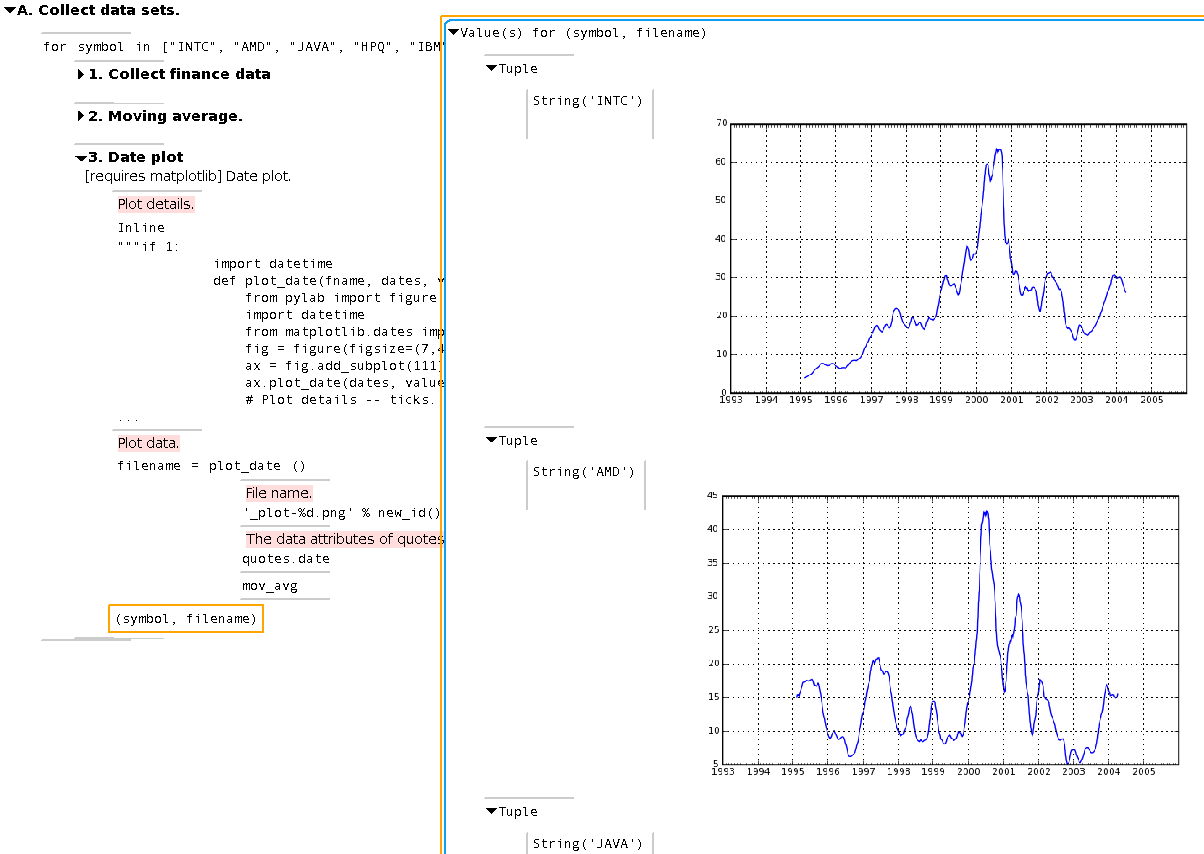
Expanding Date plot and inserting the plot data via filename shows a list of plots, but without any identifying information – not very useful yet. Instead of changing the Plot details and adding some information to the titles of the individual graphs, a simple L3 approach can be used. Insert the expression

   (symbol, filename)

after the

filename = plot_date(...) 

call and re-run the script. Note that in L3, only new or changed parts are actually executed, so re-running will not reacquire all the data. To get a table displaying the stock symbol and the graph, right-click (symbol, filename) and select insert values as l3 list. The resulting script and table look like the following.

8 Next steps

As shown, these graphs may give enough information to be useful. If so, one can next refine the plots to look better by including relevant information on them, adjusting fonts, sizes, etc. This can be done through matplotlib, using Python scripting. Even though scripting is required (a gui is not a good solution at this level of detail), it is only required for one item in the outline, the Date plot.

If more information is needed or more experimentation with these graphs is needed, more scripts can be assembled as done to this point. Unlike direct scripting, these additions can be made anywhere in the existing script, including loop bodies, and only the additions will be re-run.

9 Summary

These assembled script fragments contain necessary script details but expose them only on demand.

The simplest use is just grabbing a pre-made script, changing some values, and executing it. This is close to the field-filling approach taken by most guis, but as illustrated, users are not restricted to this.

Multiple simple scripts can be executed in order, again with simple local customizations, and passing their computed values by name. These scripts can be accumulated and assembled into a list later.

With a useful sequence of steps done for one datum, the whole sequence is inserted into a loop construct to get the same information for more data.

For more control over details within an outline, traditional textual scripting is used.

Inspection of data is always through the script, even when loops are present.

Through use of nested outlines pre-written scripts can be significantly more complex, yet have easily edited and understood components.

File names are generated and need not be changed, i.e. file naming issues can be ignored.

---

Footnotes:

¹ This example is tested using matplotlib version 0.90.1. On debian-based systems,

 apt-get install python-matplotlib python-matplotlib-data python-matplotlib-doc

will provide this.