RPy demo in L3

1 Start with the script

Starting point for this demo is the script, produced as usual via a text editor; it contains far too much detail to make graphical editing practical:

if ("outline", "External code"):
    inline '''if 1:
    from rpy import *
    d = r.capabilities()
    if d['png']:
        device = r.png 
        ext='png'
    else:
        device = r.postscript
        ext='ps'
    '''
 
if ("outline", "Parameters"):
    img_width = 400
    img_height = 300
    ed = r.faithful["eruptions"] 
 
if ("outline", "Summary of Old Faithful eruption duration data"):
    r.sink('_summary-%d.txt' % new_id())
    r.print_(r.summary(ed))
    r.sink()
 
if ("outline", "Stem-and-leaf plot of Old Faithful eruption duration data"):
    r.sink('_stemleaf-%d.txt' % new_id())
    r.stem(ed)
    r.sink()
 
if ("outline", "Old Faithful eruptions"):
    file = 'faithful_histogram-%d.%s' % (new_id(), ext)
    device(file, width=img_width, height=img_height)
    r.hist(ed,r.seq(1.6, 5.2, 0.2), prob=1,col="lightgreen",
           main="Old Faithful eruptions",
           xlab="Eruption duration (seconds)")
    r.lines(r.density(ed,bw=0.1),col="orange") 
    r.rug(ed)
    r.dev_off()
 
if ("outline", "Old Faithful eruptions longer than 3 seconds"):
    title = "Empirical cumulative distribution function of \nOld Faithful eruptions longer than 3 seconds"  
    long_ed = filter(lambda x: x > 3, ed)
    file = 'faithful_ecdf-%d.%s' % (new_id(), ext)
    device(file, width=img_width,height=img_height)
    r.library('stepfun')
    r.plot(r.ecdf(long_ed), do_points=0, verticals=1, main = title) 
    x = r.seq(3,5.4,0.01)
    r.lines(r.seq(3,5.4,0.01),
            r.pnorm(r.seq(3,5.4,0.01),
                    mean=r.mean(long_ed), sd=r.sqrt(r.var(long_ed))),
            lty=3, lwd=2, col="red")
    r.dev_off()
 
if ("outline", "Quantile plots"):
    file = 'faithful_qq-%d.%s' % (new_id(), ext)
    device(file, width=img_width, height=img_height)
    r.par(pty="s")
    r.qqnorm(long_ed, col="blue")
    r.qqline(long_ed, col="red")
    r.dev_off()
 
if ("outline", "Shapiro-Wilks normality test of Old Faithful eruptions longer than 3 seconds"):
    r.library('ctest')
    sw = r.shapiro_test(long_ed)
 
if ("outline", "One-sample Kolmogorov-Smirnov test of Old Faithful eruptions longer than 3 seconds"):
    ks = r.ks_test(long_ed,"pnorm", mean=r.mean(long_ed),
                   sd=r.sqrt(r.var(long_ed)))

2 Move the script into the worksheet

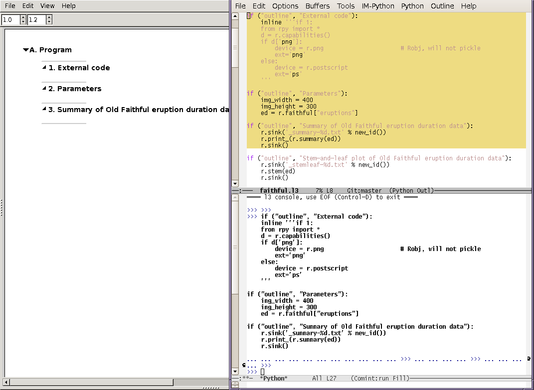
This could be loaded all at once but for exploration working with one section at a time is better. Using edit > L3 terminal console, get a console on the terminal RPy was started from. There are now three windows, the source code, the terminal, and the gui:

The gui accumulates the expressions entered into the terminal. After copying the first three outlines, this is

3 Examine key-value data

By expanding the outline, we see the three code lines; the r.sink command put plain text output into a file (which we can inspect if desired). But to just view the results, a simple menu selection is enough:

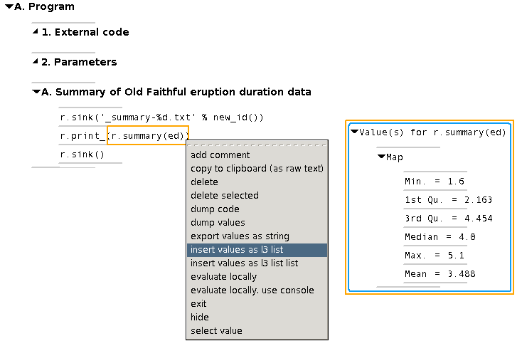
This brings the script and its output together in one place and there is no redundant information – the header describes what we're looking at, without additional print statements to provide the same information in the output.

4 View some graphs

The graphical abilities of R can be used similarly. Running the whole script first, we can selectively view plots. In the following image, we see the script section setting plot parameters on the left, with the (generated) file name and contents on the right:

Again, the script and the output are together, so we don't have to manually make the association between several graphs on one side and multiple script fragments on the other.

-----------

Footnotes:

¹ This demo requires R and RPy to be installed. Your system's package handler may provide these, e.g.

   apt-get install python-rpy

on Ubuntu or Debian GNU/Linux or

   yum install rpy

on Fedora 6 or newer systems. The self-contained L3 installer also has rules for installing these locally. The commands

   cd <path to installer>/bindings/rpy
   make install

will download, compile and "install" rpy and dependencies. Note that a FORTRAN compiler is required.

---